Cacophony for the whole family

Taking a break from my series of excerpts from Think DSP, I want to share an example I wrote to demonstrate some of the features in the thinkdsp library.  Last night I had the pleasure of listening to a grade school band, and during the breaks between sets, my mind wandered to the problem of synthesizing their unique sound.

With careful listening and consideration, I identified three important factors:

1. Some of the instruments are out of tune by as much as a half step.
2. At any point in the song, some fraction of the kids are not playing the written note, but choosing an alternative interpretation, plus or minus a major third.
3. At any time, a kid might pop an overtone, playing a note at 2, 3, 4, or even 5 times the intended frequency (look out, David Sanborn!).

I implemented these effects with this function, which takes a MIDI number representing the written note and returns the chosen frequency:

def random_freq(midi_num):

    # simulate poor tuning by adding 

    # gaussian noise to the MIDI number

    midi_num += random.gauss(0, 0.5)

    

    # one kid out of 10 plays the wrong note

    if random.random() < 0.1:

        midi_num += random.randint(-5, 5)

        

    freq = midi_to_freq(midi_num)

    

    # and one kid in 10 pops an overtone

    if random.random() < 0.1:

        freq *= random.randint(2, 5)

    return freq

To hear what it all sounds like, check out this IPython notebook.  I hope you enjoy it as much as I enjoyed last night's performance!

Think DSP Chapter 5: Autocorrelation

It's time for Chapter 5: Autocorrelation!  If you don't think autocorrelation is interesting and fun, you are mistaken.  It turns out that autocorrelation, or something like it, explains the Missing Fundamental phenomenon I presented in last week's article.

Here are links to the previous installments:

Chapter 1: Signals and Spectrums
Chapter 2: Harmonics
Chapter 3: Chirps
Chapter 4: Noise

Autocorrelation

In Chapter 5, I explain autocorrelation by starting with the statistical definition of correlation, moving on to serial correlation, then generalizing to the autocorrelation function.

Signals often represent measurements of quantities that vary in time. For example, sound signals represent air pressure varying over time.

Measurements like this almost always have serial correlation, which is the correlation between each element and the next (or the previous). To compute serial correlation, we can shift a signal and then compute the correlation of the shifted version with the original.

def corrcoef(xs, ys):
    return numpy.corrcoef(xs, ys, ddof=0)[0, 1]

def serial_corr(wave, lag=1):
    n = len(wave)
    y1 = wave.ys[lag:]
    y2 = wave.ys[:n-lag]
    corr = numpy.corrcoef(y1, y2)[0, 1]
    return corr

corrcoef is a convenience function that simplifies the interface to numpy.corrcoef, which computes the correlation coefficient.

serial_corr takes a Wave object and lag, which is the integer number of places to shift the waves.  You can think of serial_corr as a function that maps from each value of lag to the corresponding correlation, and we can evaluate that function by looping through values of lag:

def autocorr(wave):
    lags = range(len(wave.ys)//2)
    corrs = [serial_corr(wave, lag) for lag in lags]
    return lags, corrs

autocorr takes a Wave object and returns the autocorrelation function as a pair of sequences: lags is a sequence of integers from 0 to half the length of the wave; corrs is the sequence of serial correlations for each lag.

The following figure shows autocorrelation functions for pink noise with three values of β (see Chapter 4: Noise). For low values of β, the signal is less correlated, and the autocorrelation function drops toward zero relatively quickly. For larger values, serial correlation is stronger and drops off more slowly. With  β=1.2, serial correlation is quite strong even for long lags; this phenomenon is called long-range dependence, because it indicates that each value in the signal depends on many preceding values.

With that introduction, you should check out this IPython notebook, which presents this example, then uses autocorrelation to estimate the fundamental frequency of a vocal recording.

The missing fundamental: found!

The previous installment included this notebook, which presents the phenomenon of the Missing Fundamental.  It turns out that autocorrelation sheds some light on this phenomenon.  You can read an explanation in this notebook.

Next week, for people who like the math, I derive the Discrete Cosine Transform.

Think DSP Chapter 4: Noise

In my ongoing celebration of DSP month, I am posting excerpts from Think DSP, my new introduction to Digital Signal Processing.  Here are links to the previous installments:

Chapter 1
Chapter 2
Chapter 3

Today's installment is Chapter 4: Noise.  Here's how it starts:

In English, “noise” means an unwanted or unpleasant sound. In the context of digital signal processing, it has two different senses:

1. As in English, it can mean an unwanted signal of any kind. If two signals interfere with each other, each signal would consider the other to be noise.
2. “Noise” also refers to a signal that contains components at many frequencies, so it lacks the harmonic structure of the periodic signals we saw in previous chapters.

This chapter is about the the second kind.

Chapter 4 took a while for me to get organized, because I was tempted to start with "white noise", until I realized that I could not explain what white noise is without getting myself tangled up.  It is easy to generate white noise, but not easy to explain why it is "white".

It made more sense (to me, at least) to start with uncorrelated, uniform (UU) noise and then explore the spectral structure.  What we discover is that UU noise has equal power at all frequencies, on average, and that's why it's called "white".

Here's the power spectrum of a segment of UU noise.

It looks like the same power at all frequencies, on average, but it's pretty noisy.  The picture is clearer if we compute the cumulative sum of power:

That smooths out the noise and makes the "whiteness" obvious.

The chapter also presents Brownian noise (aka "red noise") and pink noise, wrapping up this this figure, which shows the power spectrums for red, pink, and white noise on a log-log scale:

You can see the examples from Chapter 4 (and listen to them) in this IPython notebook.

And if you can't wait for Chapter 5, you might be interested in this notebook, which presents the phenomenon of the Missing Fundamental.

Think DSP Chapter 3: Chirps

In my ongoing celebration of DSP month, I am posting excerpts from Think DSP, my new introduction to Digital Signal Processing.  Here are links to the previous installments:

Chapter 1
Chapter 2

Today's installment is Chapter 3, of course.  But right now I am in the process of finishing Chapter 9, which is about signals and linear, time-invariant (LTI) systems.   I just finished one of the coolest examples in the book, and I can't resist jumping ahead a little.  So, before we get to Chapter 3, please check out this IPython notebook, and then come right back.

Chapter 3

Welcome back.  I hope you like the "violin in a firing range" example, and I hope it makes you want to stick around and see how it works.  Chapter 3 might not be quite as cool, but it has some good stuff, too, like chirps and the Eye of Sauron.  Here's the introduction:

"The signals we have worked with so far are periodic, which means that they repeat forever. It also means that the frequency components they contain do not change over time. In this chapter, we consider non-periodic signals, whose frequency components do change over time. In other words, pretty much all sound signals.

"We’ll start with a chirp, which is a signal with variable frequency. Here is a class that represents a chirp:

class Chirp(Signal):
    
    def __init__(self, start=440, end=880, amp=1.0):
        self.start = start
        self.end = end
        self.amp = amp

"start and end are the frequencies, in Hz, at the start and end of the chirp. amp is amplitude."

You can see (and hear) the examples from Chapter 3 in this IPython notebook.  It includes this figure:

Which is the spectrum of a chirp that sweeps from 220 Hz to 440 Hz.  The spectrum shows a "blur" of frequencies in that range, but because of leakage, it has a cool pattern across the top that looks a little bit like this:

That's the Eye of Sauron at the top of Barad-dûr (a tower in the Lord of the Rings, in case you didn't know).

Chapter 3 also presents spectrograms, which are visualizations of the short-time Fourier transform (STFT).  A STFT breaks a wave up into short intervals and computes the Fourier transform of each interval.  The visualization shows time on the x-axis and frequency on the y-axis.  This example shows the spectrogram of a chirp that sweeps from 220 to 440 Hz:


This chapter also features one of my favorite exercises, the sawtooth chirp:

"Write a class called SawtoothChirp that extends Chirp and overrides evaluate to generate a sawtooth waveform with frequency that increases (or decreases) linearly.

"Draw a sketch of what you think the spectrogram of this signal looks like, and then plot it. The effect of aliasing should be visually apparent, and if you listen carefully, you can hear it."

This exercise has a punchline: if you implement the sawtooth chirp correctly, it should sound familiar, at least to viewers of a certain age.  Hint.

You can read the rest of Chapter 3 here.  In a few days I will post Chapter 4: Noise!

Think DSP Chapter 2: Harmonics

A few days ago I posted the first chapter from Think DSP, a new book taking a computational approach to Digital Signal Processing.  Over the next few weeks I'll post additional chapters and related blog articles.

Chapter 1 elicited some discussion on the discussion group Comp.DSP, where the focus of the conversation is the correct plural of "spectrum".  The most commonly used plural is "spectra", based on the sort-of-rule that words from Latin should use Latin plurals.  But this rule doesn't hold up very well to scrutiny, as in this video explaining why the plural of octopus would be octopodes.

So I decided to explore a radical version of an alternative rule, which is to pluralize English words using standard English endings, regardless of their etymological roots.  In Think DSP I use "spectrums";  I suspect that my former Latin teachers do not approve.

Moving on to less important matters, Chapter 2 is about the harmonic structure of certain periodic signals, and about aliasing.

Harmonics

Here's the spectrum of a triangle signal at 200 Hz.

The biggest peak is at 200 Hz, right where we expect it, but there are additional peaks at all the odd multiples of 200 Hz.  And the amplitude of those peaks is proportional to the inverse of frequency squared.

A square wave also contains odd harmonics, but they drop off more slowly, inversely proportional to frequency (not frequency squared).  A sawtooth wave contains both even and odd harmonics, and they are inversely proportional to frequency.

So that raises a question I posed in one of the exercises:  Is there a simple waveform that has even and odd harmonics that drop off like  1/ f ²?

Aliasing

The figure below shows a cosine signal at 4500 Hz sampled at 10,000 frames a second.

The figure above shows a cosine signal at 5500 Hz sampled at 10,000 frames a second.

If you compare the two figures, you'll notice the problem: at this framerate, the two signals are indistinguishable.  This result is an example of aliasing, where a signal at one frequency masquerades as another frequency.

Chapter 2 explains more about how all this works.  You can see the code and examples in

the Chapter 2 IPython notebook, and you can read the whole chapter here.

And if you want to read the rest of the book, the current draft is here:

The Think DSP web page

Think DSP is a Free Book. It is available under the Creative Commons Attribution-NonCommercial 3.0 Unported License, which means that you are free to copy, distribute, and modify it, as long as you attribute the work and don't use it for commercial purposes.

In particular, I welcome comments and suggestions from readers.  You can add a comment to this blog, or send me email.  If I make a change based on your suggestion, I will add you to the book's contributor list (unless you ask me not to).

Finally, be sure to tell me what you think the plural of "spectrum" should be.  Maybe "spectropodes"?

  

January is DSP month!

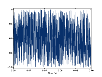
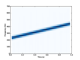
Segment of a violin recording.

I'm happy to announce that January is Digital Signal Processing month -- at least according to me.  I am planning to celebrate by publishing a sneak preview of chapters from the book I am working on, Think DSP.

Think DSP is the latest in my series Think X (for all X).  The series is based on the premise that many topics that are usually presented mathematically are easier to understand and work with computationally. 

And Digital Signal Processing is a perfect example.  In most books, Chapter 1 is about complex arithmetic, and you don't get to interesting applications for a few hundred pages, if ever.

With a computational approach, you have the option to go top-down: that is, you can start with applications, using packages like NumPy to do the computation, and for each technique, you can learn what it does before you learn how it works.

The power of this approach is clearest when you get to the exercises.  After the first chapter of Think DSP, readers can generate and listen to complex signals, download (or make) a sound recording, compute and display its spectrum, apply filters, and play back the results.  To see what I am talking about, check out this IPython notebook, which contains the examples from Chapter 1:

Chapter 1 Notebook

I think it's a lot more fun than the usual approach.

If you know a little bit about signal processing, you can probably understand the material in the notebook.  But if you're a beginner, you should read Chapter 1 first.  Here's an excerpt:

"A signal is a representation of a quantity that varies in time, or space, or both. That definition is pretty abstract, so let’s start with a concrete example: sound. Sound is variation in air pressure. A sound signal represents variations in air pressure over time.

"A microphone is a device that measures these variations and generates an electrical signal that represents sound. A speaker is a device that takes an electrical signal and produces sound. Microphones and speakers are called transducers because they transduce, or convert, signals from one form to another.

"This book is about signal processing, which includes processes for synthesizing, transforming, and analyzing signals. I will focus on sound signals, but the same methods apply to electronic signals and mechanical vibration.

"They also apply to signals that vary in space rather than time, like elevation along a hiking trail. And they apply to signals in more than one dimension, like an image, which you can think of as a signal that varies in two-dimensional space. Or a movie, which is a signal that varies in two-dimensional space and time.

"But we start with simple one-dimensional sound."

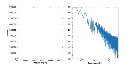
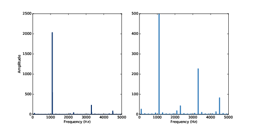
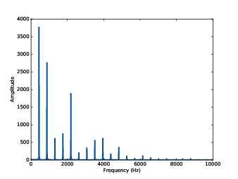
Spectrum of a segment from a violin recording.

You can read the rest of the chapter here:

Chapter 1 in HTML

And if you want to read the rest of the book, the current draft is here:

The Think DSP web page

Think DSP is a Free Book. It is available under the Creative Commons Attribution-NonCommercial 3.0 Unported License, which means that you are free to copy, distribute, and modify it, as long as you attribute the work and don't use it for commercial purposes.

In particular, I welcome comments and suggestions from readers.  You can add a comment to this blog, or send me email.  If I make a change based on your suggestion, I will add you to the book's contributor list (unless you ask me not to).